Defect – Definition

This post presents ITU-T G.806’s definition of a defect or defect condition.

Defect – Definition

ITU-T G.806 defines the word defect as follows:

Defect: The density of anomalies has reached a level where the ability to perform a required function has been interrupted.

We use defects as an input for performance monitoring, controlling consequent actions, and determining fault causes.

In other words, defects are bad.

If some piece of networking equipment is declaring a defect condition, it is saying it “cannot do its job properly” because of this condition.

Defects that We Cover in this Blog

We cover the following defects in this blog.

For OTN Applications

OTU Layer
  • dLOS-P – Loss of Signal – Path
  • dLOS-P[i] – Loss of Signal – Path, Electrical Lane, i
  • dLOFLANE[j] – Loss of Frame – of Logical Lane j
  • dLOR[j] – Loss of Recovery, Logical Lane j
  • dLOL – Loss of Lane Alignment
  • Excessive Skew (OTL3.4 and OTL4.4 Applications)
  • dLOF – Loss of Frame
  • dLOM – Loss of Multi-Frame
  • dAIS – (OTUk-) Alarm Indication Signal
  • dTIM – Trail Trace Identifier Mismatch
  • dBDI – Backward Defect Indicator
  • dDEG – Signal Degrade
  • dIAE – Input Alignment Error
  • dBIAE – Backward Input Alignment Error
ODU Layer
  • dAIS – (ODUk) Alarm Indication Signal
  • dLCK – Locked Status
  • dOCI – Open Connection Indication
  • dTIM – Trail Trace Identifier Mismatch
  • dBDI – Backward Defect Indicator
  • dDEG – Signal Degrade
Non-Multiplexed Applications
  • dLCS – Loss of Character Synchronization (100GBASE-R)
  • dPLM – Payload Type Mismatch
Multiplexed Applications
  • dLOOMFI – Loss of OMFI Synchronization
  • dLOFLOM[p] – Loss of Frame, Loss of Multi-Frame – ODUj Tributary Port p
  • dMSIM[p] – Multiplex Structure Identifier Mismatch – ODUj Tributary Port p
Tandem Connection Monitoring (TCM)
  • TCMi-dAIS – TCM Level i, Alarm Indication Signal
  • TCMi-dLCK – TCM Level i, Locked Status
  • TCMi-dOCI – TCM Level i, Open Connection Indication
  • TCMi-dTIM – TCM Level i, Trail Trace Identifier Mismatch
  • TCMi-dBDI – TCM Level i, Backward Defect Indicator
  • TCMi-dDEG – TCM Level i, Signal Degrade
  • TCMi-dIAE – TCM Level i, Input Alignment Error
  • TCMi-dBIAE – TCM Level i, Backward Input Alignment Error
  • dLTC – Loss of Tandem Connection Monitoring

Clueless about OTN? We Can Help!!! Click on the Banner Below to Learn More.

Discounts Available for a Short Time!!!

What is Full-Duplex Communication?

This post briefly defines Full-Duplex Communication. It also highlights differences between Full-Duplex and Half-Duplex Communication.


What is Full-Duplex Communication?

We define Full-Duplex Communication as communication occurring in both directions simultaneously.

Some Communications Literature will use the abbreviation FDX to denote Full-Duplex Communication.

A couple of examples of Full-Duplex Communications would be Cellular Phones and much of modern internet-based communication services (e.g., Video Communication via Skype, Face-Time, etc.).

Two women demonstrating Full-Duplex communications via cell phones.
Isolated portrait of two teenage girls with cell phones

We have the bandwidth (or a communications channel) available in these technologies in both directions.

Unlike Half-Duplex Communication, there is no means (or need) to control access to a single communications channel.

Each direction has its own communications channel and can communicate freely, at will, or whenever data is available.

An Analogy for Full-Duplex Communications

We can think of Full-Duplex Communications as being just like a two-way street on the roadways.

A Freeway is a good analogy to Full-Duplex Communications

Most modern forms of communication we use today (e.g., cell phones or tablets engaging in video conferencing, or just communicating with websites – for gaming, social media, etc.) all use Full-Duplex Communications.

In the old days, Ethernet started using Half-Duplex communications (for 10BASE-T, etc.)  However, once Ethernet moved on to faster speeds and began to use switching technology, it started supporting Full-Duplex communications.

Other forms of Communication types include:

Has Inflation got You Down? Our Price Discounts Can Help You Beat Inflation and Help You Become an Expert on OTN!! Click on the Banner Below to Learn More!!

Discounts Available for a Short Time!!

What is Half-Duplex Communication?

This post briefly defines the term: Half-Duplex Communication.


What is Half-Duplex Communication?

We define Half-Duplex Communication as communication occurring in both directions but in only one direction at a time.

Some Communications Literature will use the abbreviation HDX to denote Half-Duplex Communication.

Some examples of Half-Duplex Communications systems would be Speakerphones or Walkie-Talkies.

A speakerphone is an example of Half-Duplex Communication

In both examples, legible communication can only flow if only one side is talking and the other direction (or side) is silent.

Controlling the Communication

In Half-Duplex Communication systems, there must be some control (or protocol) that decides which side (or direction) gets to transmit their information or data at a given time.

In the case of speakerphones or walkie-talkies, there needs to be some agreement (or understanding) among human beings (on both ends of the connection) on who gets to speak and when.

For electronic or automatic half-duplex systems, electronic circuitry controls which side gets to communicate or use the “channel,” when and for how long.

We will typically use Half-Duplex Communication to:

  • Support bi-directional communication, and
  • Conserve bandwidth (both directions use the same channel or bandwidth).

What are the Differences between Simplex and Half-Duplex Communication?

Half-Duplex communication is similar to Simplex Communication in that communication can only occur in one direction at a time.

However, Half-Duplex communication is different from Simplex Communication in that it also supports communication in the other direction.

It just doesn’t support bi-directional communication simultaneously.  That would be Full-Duplex Communication.

Another Example?

A good analogy for Half-Duplex Communication would be with a road construction scenario.  Consider the case where there is only one lane available to two-way traffic (over a bridge – for example).

Road Construction is an example of Half-Duplex Communication

In this case, traffic controller personnel (with signs) would be deciding and controlling which direction gets to use the available lane.  In the meantime, traffic in the other direction has to wait until they get the “go ahead” from the traffic controllers.

Other forms of Communication types include:

Has Inflation got You Down? Our Price Discount Can Help You Beat Inflation and Help You Become an Expert on OTN!! Click on the Banner Below to Learn More!!!

Discounts Available for a Short Time!!!

What is Simplex Communication?

This post briefly defines the term: Simplex Communication.


What is Simplex Communication?

We define simplex communication as communication that only operates in one direction.

Simplex is One Way or One Direction Communication

A couple of obvious examples of Simplex Communication would be Radio or Television Broadcasting.

Satellite Dish receives One-Way Communication (or Broadcasts) from Radio/TV Stations
Satellite dish on the modern building roof corner with blue sky in the background.

Unless you count being able to place a phone call to your Radio or TV Station, you can’t usually send traffic back to the Radio or TV Station transmitter.

ITU (International Telecommunication Union) defines Simplex Communication as a communication channel that operates in one direction at a time but maybe reversible (communication can occur in the opposite direction).

I would argue that ITU’s definition is that for Half-Duplex Communication.

Other basic terms for communications include:

Has Inflation got You Down? Our Price Discount Can Help You Fight Inflation and Help You Become an Expert on OTN!! Click on the Banner Below to Learn More!!!

Discounts Available for a Short Time!!!

What is the Wait-to-Restore Period?

This post briefly defines and describes the term Wait-to-Restore for Protection-Switching systems.


What is the Wait-to-Restore Period within a Protection-Switching System?

The purpose of this post is to describe and define the Wait-to-Restore period within a Revertive Protection-Switching system.

Introduction

All Protection Groups will perform Protection-Switching, to route the Normal Traffic Signal around a defective Working Transport entity anytime it is declaring a service-affecting or signal degrade (dDEG) defect with that Working Transport entity.

In other words, the Protection Group will route the Normal Traffic Signal through the Protection Transport entity for the duration it declares this defect condition.

Whenever a Revertive Protection Group clears that defect, it will switch the Normal Traffic Signal back to flowing through the Working Transport entity.

We call this second switching procedure (to return the Protection-Group to its NORMAL, pre-protection-switching state) revertive switching.

In contrast, a Non-Revertive Protection Group will NOT perform this revertive switch, and the Normal Traffic Signal will continue to flow through the Protection Transport entity indefinitely.

When the Tail-End Node clears the Service-Affecting Defect

Protection-Switching events are very disruptive to the Normal Traffic Signal.  Each time we perform a protection-switching procedure, we induce a glitch (or a burst of bit errors) and signal discontinuity within the Normal Traffic Signal.

Therefore, Protection-Switching events should not be a common occurrence within any network.

To minimize the number of protection-switching events (occurring within a network), the Protection-Group will usually force the Tail-End Node to go through a Wait-to-Restore period after it clears the service-affecting or dDEG defect (which caused the Protection-Switching event in the first place) before it can proceed on to the next step and revert the protection-switching (and traffic).

In other words, the Tail-End Node (within a Protection-Group) will execute the following steps each time it clears a defect, which causes a protection-switching event.

  1. It clears the defect condition.
  2. The Tail-End circuit will then start a Wait-to-Restore Timer and will wait until this timer expires before it proceeds to the next step.
  3. If the Tail-End circuit declares another service-affecting defect while waiting for this Wait-to-Restore timer to expire, it will reset this timer back to zero and continue waiting.
  4. Once the Wait-to-Restore timer expires, the Tail-End circuit will revert the protection-switched configuration into the NORMAL configuration.  In other words, the Normal Traffic Signal will (once again) travel along the Working Transport entity.  

I show these same steps within the Revertive Procedure Flow Chart below.

Revertive Protection Switching Procedure Flow Chart

Figure 1, Flow-Chart of the Revertive Protection-Switching Procedure – after the Service-Affecting defect clears.

What is the purpose of using this Wait-to-Restore Period?

There are two main reasons why we use the Wait-to-Restore period in a Protection-Switching system.

  1. To make sure that the condition of the Working Transport entity has stabilized and is not still declaring intermittent defects before we start to pass the Normal Traffic signal through it again.
  2. And to reduce the number of protection-switching events within a protection group.

How Long Should the Wait-to-Restore period be?

ITU-T G.808.1 recommends that this period be between 5 and 12 minutes.

In Summary

All revertive protection-switching systems must wait through a Wait-to-Restore period (after clearing the defect condition) before executing the revertive switch.

The purpose of waiting through this Wait-to-Restore period is to prevent multiple Protection-Switching events due to intermittent defects within the Working Transport entity.

ITU-T G.808.1 recommends that this Wait-to-Restore period be between 5 and 12 minutes.

This means that the Tail-End circuit must go through this Wait-to-Restore period and declare no defects for the entire 5 to 12-minute period before it can move on to revert its protection-switching.

Has Inflation got You Down? Our Price Discounts Can Help You Beat Inflation and Become an Expert on OTN!! Click on the Banner Below to Learn More!!

Discounts Available for a Short Time!!!

For More Information on other Protection-Switching-related Posts, Click on the Image Below.

Protection-Switching Related Blog

Protection-Switching Related Blog Posts

Protection-Switching Related Blog Posts Basic Protection-Switching Terms Head-End (Source Node) Hold-Off Timer Protection-Group Protection-Transport entity Selector Switch Tail-End (Sink Node) ...

What is a Revertive APS System?

This post briefly defines and describes Revertive Protection Switching.

What is a Revertive APS (Automatic Protection-Switching) System?

If an Automatic Protection System is Revertive, then that means that the system will always return to transmitting/accepting the Normal Traffic Signal through the Working Transport Entity anytime the system has recovered from a defect or an external request (for Protection Switching).

An Example of Revertive Switching

Let’s use an example to help define the term revertive.

The Normal/No Defect Case

Let’s consider a 1:2 Protection Switching System shown below in Figure 1.

Linear Protection Switching - 1:2 Protection-Switching Architecture

Figure 1, Illustration of a 1:2 Protection Switching System – West to East Direction

NOTE:  Because the 1:N Protection-Switching pictures are somewhat complicated, I only show the West-to-East Direction of this Protection-Switching system to keep these figures simple.

In Figure 1, all is well.  Both of the Normal Traffic Signals within the figure (e.g., Normal Traffic Signal # 1 and Normal Traffic Signal # 2) flow from their Head-End Nodes to their Tail-End Nodes with no defects or impairments.

The Defect Case

Let’s assume that an impairment occurs within Working Transport Entity # 1 and that the Tail-End circuitry (associated with Working Transport Entity # 1) declares either a Service-Affecting or Signal Degrade Defect (e.g., declares the SF or SD condition).

We show this scenario below in Figure 2.

1:2 Protection Switching Scheme - Defect in Working Transport entity # 1

Figure 2, Illustration of our 1:2 Protection-Switching system (West to East Direction only) with a Service-Affecting Defect occurring in Working Transport Entity # 1 

The Protection-Switch

Whenever the Tail-End circuitry (within Figure 2) declares the service-affecting defect condition, it will (after numerous steps) achieve the Protection-Switching configuration shown below in Figure 3.

1:2 Protection Switching Scheme - Protection Event

Figure 3, Illustration of our 1:2 Protection-Switching system (West to East Direction only) following Protection-Switching.

NOTE:  Check out the post on the APS Protocol (within “THE BEST DARN OTN TRAINING PERIOD” training sessions) to understand the sequence of steps that the Tail-End and the Head-End Nodes had to execute to achieve the configuration we show in Figure 3.

Our 1:2 Protection-Switching system will remain in the condition shown in Figure 3 for the duration that the Tail-End Circuitry declares this defect within Working Transport Entity # 1.

The Defect Clears

Eventually, the Service-Provider will roll trucks (e.g., send repair personnel out to fix the fault condition, causing the service-affecting defect); and the defect will clear.

Once this service-affecting defect clears, the East Network Element will wait some WTR (or Wait-to-Restore) period before it proceeds with the Revertive switch.

Clueless about OTN? We Can Help!!! Click on the Banner Below to Learn More!!!

Corporate Discounts Available!!

The Revertive-Switch

Once the WTR period expires (with no further defects occurring within Working Transport Entity # 1), our Protection Group will switch and route Normal Traffic Signal # 1 back through Working Transport Entity # 1.

We show the resulting configuration below in Figure 4.

Linear Protection Switching - 1:2 Protection-Switching Architecture

Figure 4, Illustration of our 1:2 Protection-Switching System (West to East Direction ONLY) following Revertive-Switch

The Overall Flow for Revertive Switching

Figure 5 presents a flow-chart diagram that summarizes the Revertive Protection-Switching Procedure.

Revertive Protection Switching Procedure Flow Chart

Figure 5, Flow-Chart Diagram summarizing the Revertive Protection Switching Procedure

Check out the relevant post for more information about the Wait-to-Restore period and Timer.

In Summary

A Revertive Protection-Switching system will always perform a second switching procedure after the defect has cleared.

This second switching procedure will return the Protection Group to the state of having the Normal Traffic Signal flowing through the Working Transport Entity.

A Non-Revertive Protection-Switching system will NOT perform this second switching after the Tail-End Node has cleared the service-affecting defect.

Therefore, in a Non-Revertive Protection-Switching system, the Normal Traffic Signal will continue to flow through the Protection Transport entity indefinitely.

To use a Revertive Protection-Switching System or NOT.

There are advantages and disadvantages to using a Revertive system.

I list some of these advantages and disadvantages below.

Disadvantages of Using a Revertive System

  • Each service-affecting or signal degrade defect (SD or SF) occurrence will result in two Switching Events.  We will disrupt the Normal Traffic Signal twice for each defect condition.
    • The first switching event is in response to the defect condition, and
    • The follow-up Revert Switching event.

We strongly advise that you use Revertive Protection-Switching if:

  • You are using a Shared-Ring Protection-Switching system.
  • If the Bandwidth or Performance Capability of the Protection Transport entity is lower or worse than that for the Working Transport Entity (e.g., has more bit errors, inferior performance)
  • Whenever there is a much more significant delay in the Protection Transport entity (than that for the Working Transport entity)
  • If one needs to track which Protected ports are using the Working Transport entity and which are using the Protection Transport entities
  • Protection Transport entity must be readily available for multiple other Working Transport entities (as in a 1:N Protection Architecture).

Has Inflation got You Down? Our Price Discounts Can Help You Beat Inflation and Help You to Become an Expert on OTN!! Click on the Banner Below to Learn More!!!

Discounts Available for a Short Time!!!

Click on the Image Below to see more Protection-Switching related content on this Blog:

Protection-Switching Related Blog

Protection-Switching Related Blog Posts

Protection-Switching Related Blog Posts Basic Protection-Switching Terms Head-End (Source Node) Hold-Off Timer Protection-Group Protection-Transport entity Selector Switch Tail-End (Sink Node) ...

Linear Protection Switching

This post briefly defines the term: Linear Protection Switching. It also briefly defines 1+1, 1:N Protection Architectures.


What is Linear Protection Switching?

A Linear Protection-Switching System is a Protection System (or Protection Group) that contains two nodes:

Each of these two nodes is exchanging normal traffic signals, with each other, over a protected network that consists of both the Working Transport entity and the Protect Transport entity.

I show some simple pictures of Linear Protection Switching Systems below in Figures 1, 2, and 3.

The 1+1 Protection-Switching Architecture

1+1 Linear Protection-Switching System

Figure 1, Illustration of a Linear Protection Switching System (A 1+1 Protection-Switching System)

In Figure 1, I show a simple illustration of a 1+1 Protection-Switching system, which also presents the bidirectional traffic flow between the Head-End and Tail-End Nodes.

If you want to learn more about the 1+1 Protection-Switching Architecture, check out the post on this topic.

The 1:N Protection-Switching Architecture

Linear Protection Switching - 1:2 Protection Switching Architecture

Figure 2, Illustration of a Linear Protection Switching System (A 1:2 Protection-Switching System) – for the East to West Direction

Linear Protection Switching - 1:2 Protection-Switching Architecture

Figure 3, Illustration of a Linear Protection Switching System (A 1:2 Protection-Switching System) – for the West to East Direction

Figures 2 and 3 each present an illustration of a 1:2 (or 1:N) Protection-Switching System.

Please note that the 1:N Protection-Switching Architecture figures are more complicated than that for the 1+1 Protection-Switching Architecture.

Therefore, I needed to show this architecture in the form of two figures. 

One figure shows the traffic flowing from West to East, and the other illustrates the traffic flowing from East to West.

If you want to learn more about the 1:2 (or 1:N) Protection-Switching architecture, check out the post on that topic.

In summary, the 1+1 and the 1:N Protection-Switching schemes are Linear-Protection Protection-Switching systems.

Design Variations for Linear Protection-Switching Systems

Linear  Protection-Switching systems are available in a wide variety of features.  I’ve listed some of these features and their variations below.

Architecture

Switching Type

Operation Type

APS Protocol – Using the APS/PCC Channel

Click on any of the links above to learn more about these design variations within a Linear Protection-Switching System.

What about Other Protection-Switching Architectures?

There are other types of Protection Switching systems, which are not Linear, such as Shared-Ring Protection-Switching or Shared-Mesh Protection-Switching.

Please see the relevant posts for more information about those types of Protection-Switching Systems.

Has Inflation got You Down? Our Price Discounts Can Help You Beat Inflation and Help You to Become An Expert on OTN!!! Click on the Banner Below to Learn More!!!

Discount Available for a Short Time!!

Click on the Image Below to see more Protection-Switching related content on this Blog:

Protection-Switching Related Blog

Protection-Switching Related Blog Posts

Protection-Switching Related Blog Posts Basic Protection-Switching Terms Head-End (Source Node) Hold-Off Timer Protection-Group Protection-Transport entity Selector Switch Tail-End (Sink Node) ...

What is Running Disparity (RD)?

The Running Disparity (or RD) is defined as the difference between the number of logic 1 bits and logic 0 bits between the start of a data sequence and a particular instant in time during its transmission.


What is Running Disparity (RD)?

We define the Running Disparity (or RD) as the difference between the number of logic 1 bits and logic 0 bits between the start of a data sequence and a particular instant in time during its transmission.

In other words, the RD for a character is the difference between the number of logic 1 bits and logic 0 bits in that character.

Hence, if there are more logic 1 bits than logic 0 bits (within a character or string of consecutive bits), we can state that the RD is positive.

If there are more logic 0 bits than logic 1 bits, then we can state that the RD is negative.

Finally, if the number of logic 1 and logic 0 bits are the same, we can state that the RD is neutral or zero.

We can express the Running Disparity as either an integer or as a ratio:

EXPRESSING RD AS AN INTEGER NUMBER:

If you wish to express the RD of a character or string (of consecutive bits) as an integer number, then you can calculate the RD with the following equation:

RD = (Number of Logic 1 bits in the character or string) – (Number of Logic 0 bits in the character or string)

For example:  

The running disparity of the hexadecimal expression of 0x78 is 0.

To understand why this is the case, if we were to express this value in its binary format, we get 0111 1000.  The binary expression (for this value) contains four 0s and four 1s.

Thus, RD = 4 – 4 = 0

On the other hand, the running disparity of the hexadecimal expression of 0x7F is +6.

Again, if we were to express this value in its binary format, we would get 0111 1111.  The binary expression (for this value) contains seven 1s and one 0.

Hence, RD = 7 – 1 = +6

EXPRESSING RD AS A RATIO:

If you wish to express the RD of a character or string (of consecutive bits) as a ratio, then you would do the following:

  • Count the total number of logical “1s” in the expression.
  • Count the total number of logical “0s” in the expression.

And then express this information in the following format:

Number of Logical 1s (in character/string) :  Number of Logical 0s (in character/string)

For example:

We express the running disparity of the hexadecimal expression of 0x78 as:

4:4, which we can reduce (or simplify) to 1:1.

Likewise, we can compute and express the RD for the value 0x7F as
7:1.

Some communication and data storage system standards (such as Gigabit Ethernet/1000BASE-X, Fibre-Channel, etc.) require that we maintain the RD as near to neutral as possible.

The system designer must ensure that the ratio of logical 1 bits to logical 0 bits (over time) should be kept close to 1:1.

Thus, the System Designer must follow any character/string with negative disparity with another character/string with an equal amount of positive disparity, and vice-versa.

Keeping RD to a minimum is to maintain dc balance on the transmission medium.

The System Designer must ensure that the RD does not increase without bounds.

The 8B/10B line code is a specific example of a line code that requires and exercises control over RD.

NOTE:  Controlling and monitoring RD can also help detect transmission errors.

Has Inflaton got You Down? Our Price Discounts Can Help You Fight Inflation and Help You Become an Expert on OTN!! Click on the Banner Below to Learn More!!

Discounts Available for a Short Time!!!

Manchester Encoding

This post presents a description of the Manchester Line Code. It also describes the Manchester Line Code’s strength, weaknesses and where it is deployed.

What is the Manchester Line Code

The Manchester Line Code is a line code that transports both data and timing information on a single serial binary data stream.

We use the Manchester Line Code in the Physical Layer.

A Manchester Line Encoder works by encoding each data bit to be either low-then-high or high-then-low – for equal amounts of time.  

Since this encoded data is “high” and “low” for equal times, there is no DC bias within this signal.

More specifically, IEEE 802.3 specifies that a Manchester encoder should encode a “1” bit by setting the output to a logic “low” for the first half of a bit period and then by setting the output to a logic “high” for the second half of this bit period.  

This encoding scheme requires a rising clock edge at the middle of this bit period.  

Conversely, IEEE 802.3 also specifies that a Manchester encoder should encode a “0” bit by setting the output to a logic “high” during the first half of a bit period and then set the output to a logic “low” for the second half of the bit period.  

This situation requires a falling clock edge to occur in the middle of this bit period.

Figure 1 shows a drawing of a data stream that we have encoded into the Manchester format.  

The very top trace is the clock signal.  The middle signal trace contains the data (that we wish to encode).  Finally, the bottom signal trace presents the resulting encoded data.

Manchester Line Code

Figure 1, An Drawing of a Data Stream that we have encoded into the Manchester format

Manchester coding works by exclusive-ORing (XOR) the Original Data and the Clock signal, as Table 1 presents below.

Table 1, Encoding Data into the Manchester Line Code

Manchester Encoding Algorithm

Where did the Manchester Line Code come from?  

The University of Manchester (in the United Kingdom) developed the Manchester Line Code.

What are its strengths?  

The Manchester Line Code has two primary strengths:

  1. It is an electrically balanced line code and has no DC bias.
  2. It provides many clock edges for “clock and data recovery” at the remote receiving terminal.  The Manchester Line Code does not need to use any “Zero-Suppression” scheme.

What are its weaknesses?  

Since Manchester encoding requires a clock edge for each bit of data, the frequency content of a Manchester-encoded signal is relatively high.  

This fact limits the data rates at which the user can transmit a Manchester encoded data stream over a band-limited channel.  

In other words, the Manchester line code is not suitable for transmitting high-speed signals over band-limited channels.

Where is it used?  

10BASE-T (10Mbps Ethernet over Twisted Pair) applications use the Manchester Line Code.

Other Line Codes

  • RZ (Return to Zero)
  • NRZ (Non-Return to Zero)
  • NRZI (Non-Return to Zero-Inverted)

Stuck at Home? You Can Be an Expert on OTN Before You Return to Your Office!! Click on the Banner Below to Learn More!!

Discounts Available for a Short Time!!

The Physical Layer – within the OSI Reference Model

This post presents a discussion of the Physical Layer, within the OSI Reference Model.


What is the Physical Layer – within the OSI Reference Model?

The Physical Layer is the lowest-level layer within the OSI Reference Reference Model.

Figure 1 illustrates the OSI Reference Model, with the Physical Layer circled.

osi_reference_model-physical-layer

Figure 1, Illustration of the OSI Reference Model – with the Physical Layer circled

In short, a Physical Layer design focuses on transmitting a continuous data stream from one terminal to an adjacent terminal.  

As far as the Physical Layer is concerned, this data will be in the form of electrical signal pulses and optical or RF symbols – depending upon whether the communication media is copper, optical fiber, or wireless/RF.  

Additionally, Physical Layer designs/processes do not pay attention to framing or packet delineation.  

The Higher-Layer processes will handle framing and packets.  The Physical Layer processes will consider this stream of pulses to be just an unframed raw stream of bits.

Some Terminology

Throughout this blog, we will refer to the entity (e.g., the Transmitter and Receiver) that handles the Physical Layer functions (or processes) as the Physical Layer Controller.  

A transceiver is a typical example of a Physical Layer Controller.

Purpose

The purpose of the Physical Layer Controller is to provide a communications service for the local Data Link Layer Controller.  

A Physical Layer controller (at a transmitting terminal) will accept data from the local Data Link Layer Controller.  

The Physical Layer controller will transmit this data over some medium (e.g., copper, optical fiber, or wireless communication) to a similar Physical Layer Controller at the adjacent receiving terminal.  

The Physical Layer Controller (at the receiving terminal) will then provide this received/recovered data to its local Data Link Controller for further processing.

We often refer to this communication between the two Physical Layer controllers as “peer-to-peer communication” between two Physical Layer controllers.

Figure 2 presents a closer look at the physical layer controllers’ role in the transport of data.

physical_layer_processes

Figure 2, A Simple Illustration of the role that the Physical Layer controller plays in the transport of data across a media

Whenever a Physical Layer Controller (at a transmitting terminal) accepts data from the local Data Link Layer controller, it will encode it into some line code or modulation format suitable for the communication media.  

Afterward, the Physical Layer controller will transmit this data over the communication media.  

The Physical Layer controller (at the receiving terminal) will receive and recover this data from the media. 

Additionally, the Physical Layer controller will decode this data (from the line-code or modulation format) back into its original data stream.  

The Physical Layer controller will then pass this data to the Data Link Layer controller for further processing.

NOTES:

  1. Figure 2 is a simple illustration and does not include all possible circuitry within a Physical Layer controller (or Transceiver).
  2. Please see the post on the Data Link Layer for further insight into how the Data Link Layer handles this data.

Physical Layer Types in various types of Communication Media

The Physical Layer is designed to transport data from a transmitting terminal to a receiving terminal.  

The Physical Layer can be designed to transport data over any of the following types of media.

  • Copper Medium
    • Twisted-Pair
    • Coaxial Cable
    • Microstrips or Striplines on a High-Speed Backplane
  • Optical Fiber
    • Multi-Mode Fiber
    • Single-Mode Fiber
  • Wireless/RF
    • Microwave
    • Cellular
    • Satellite Communication

Physical Layer Design Considerations for Copper Media

For copper media, the Physical Layer will be concerned with the following design parameters

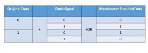
  • Line-Code (e.g., Manchester, B3ZS, 64B/66B coding, various forms of scrambling, etc.).
  • Voltage Levels of the signal (being transmitted)
    • What kind of signal/pulse should a Physical Layer controller generate and transmit to send a bit/symbol with the value of “0”?
    • The kind of signal/pulse should a Physical Layer controller generate and transmit to send a bit/symbol with the value of “1”.
    • The minimum voltage level the Receiving Physical Layer controller will correctly interpret a given bit (or symbol) as being a “1”?
    • What is the maximum voltage level for the Receiving Physical Layer controller to correctly interpret a given bit (or symbol) as being a “0”?
  • Impairments in copper media
    • Frequency-dependent loss and phase distortion of symbols.
    • Reflections
    • Crosstalk Noise
    • EMI (Electromagnetic Interference).
  • What is the maximum length of copper media that we can support?

Physical Layer Design Considerations for Optical Fiber

For an optical fiber, the Physical Layer will be concerned with the following design parameters

  • What kind of symbol are we using to transmit a bit with the value of “0”?
  • What kind of symbol are we using to transmit a bit with the value of “1”?
  • Modulation scheme (e.g., QPSK, 16QAM, PAM4, etc.)
  • What wavelength (or set of wavelengths will we use for communication)?
  • Will we transport data over single or multiple wavelengths (e.g., Wave-Division Multiplexing)?
  • Impairments in Optical Fiber
    • Chromatic Dispersion
    • Modal Dispersion (for Multi-Mode Fiber only)
    • Polarization Mode Dispersion
  • What is the maximum length of optical fiber that we can support?

Physical Layer Design Considerations for all Media

The Physical Layer will be concerned with the following design parameters, regardless of the communication media.

  • Are we transporting multiple bits via each symbol (e.g., for PAM4, 16QAM, QPSK, etc.)?
  • Bit-Timing (Bit Width) or Symbol-Timing (Symbol Width)
  • Jitter/Wander Requirements
    • Maximum allowable jitter within a transmitted signal
    • Maximum jitter tolerance capability of a receiving terminal
  • Minimum permissible SNR (Signal-to-Noise Ratio)
  • The maximum permitted BER (Bit-Error Rate)
  • Error Detection or Error Detection and Correction
  • We are ensuring a Sufficient number of transitions (in the signal waveform) to permit a CDR (Clock and Data Recovery) PLL (at the receiving terminal) to acquire and maintain lock with the incoming signal.
  • Mechanical Issues (such as connector types)
  • Whether the communication is Simplex, Half-Duplex, or Full-Duplex Mode.

The Physical Layer in other Standards

Many of the other Reference Models (e.g., OTN, SONET, SDH, and PCIe) also have a Physical Layer.  

Other postings will discuss the Physical Layer for each of these Reference Models.

You can access the posting for the Physical Layers of each of these Reference Models by clicking on the links below:

  • OTN
  • SONET
  • SDH
  • PCIe

Clueless about OTN? We Can Help!! Click on the Banner Below to Learn More!!

Discounts Available for a Short Time!!!