This blog posts highlights differences between OTN and SONET/SDH. It also provides links to other blog posts that focus on these differences in detail.
SONET/SDH and OTN are standard protocols for transporting signals from Point A to Point B on (mostly) optical fiber.
However, there are some key differences:
OTN (at least for OTU1 through OTU4) has a fixed frame size. SONET/SDH does not.
SONET/SDH has a fixed frame repetition rate (8000 frames/sec). OTN does not.
When mapping/muxing lower-speed tributary signals into higher-speed signals, SONET/SDH requires that all the lower-speed tributary signals be synchronous with each other and with the high-speed server signal. OTN does not need this.
OTN has a standard FEC (Forward Error Correction) mechanism. SONET/SDH does not have such a thing.
OTN offers more extensive TCM (Tandem Connection Monitoring) support than does SONET/SDH.
The SONET/SDH standards only support data rates of up to 40Gbps (or OC-768). The OTN standards support over 100Gbps (e.g., 200Gbps, 400Gbps, etc.)
The mechanisms for handling rate differences are handled differences between the two standards. SONET/SDH relies exclusively on something called “pointer processing.” OTN uses different mechanisms altogether (Bit Synchronous Mapping, Asynchronous Mapping, and the Generic Mapping Procedure).
Additional Questions (Topics) to be Answered in the Differences between OTN and SONET/SDH
How does SONET/SDH support TCM?
How does OTN support TCM?
What is the framing format B100G OTN?
What are the roles of the Individual Overheads Bytes for SONET/SDH? How are they different from that for OTN?
How do you map 3 STS-1 signals into an STS-3 signal? How is this different from mapping ODU1s into an ODU2?
This blog post defines the contents within the Trail Trace Identifier Messages, that we transport throughout the Optical Transport Network.
What is the Trail-Trace Identifier (TTI) Message?
We transport Trail Trace Identifier (TTI) messages at the OTU Layer, the ODU Layer, and for the (as many as 6) TCM Layers. In this blog post, I will talk about the type of data we transport within TTI Messages.
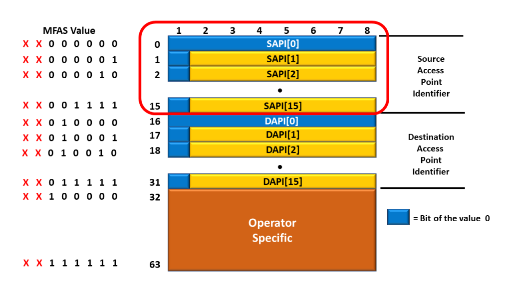
I illustrate the byte format of the Trail-Trace Identifier (TTI) message below in Figure 1.
Figure 1, Illustration of the Byte Format of the Trail-Trace Identifier (TTI) Message
Figure 1 shows that the Trail-Trace Identifier message is:
64 bytes in length,
It consists of the following fields:
16 bytes of SAPI (Source Access Point Identifier)
16 bytes of DAPI (Destination Access Point Identifier), and
32 bytes of Operator Specific data
We always synchronize our transmission of the TTI Messages with the MFAS byte.
This means that we always transmit the first byte of the SAPI field (SAPI[0]) whenever the six LSBs of the MFAS value are [0, 0, 0, 0, 0, 0], and
We transmit the last (or 64th byte of the TTI Message) whenever the six LSBs of the MFAS value are [1, 1, 1, 1, 1, 1].
Hence, we not only show the byte format of the Trail-Trace Identifier Message (in Figure 1), but we also show the sequence in which we transmit the byte within the TTI Message.
What Does SAPI (or Source Access Point Identifier) and DAPI (Destination Access Point Identifier) Mean?
The SAPI is a 16-byte sequence (or a subset of data) within the TTI Message.
The first byte of the SAPI field (SAPI[0]) is always set to 0x00.
The remaining 15 bytes (e.g., SAPI[1] to SAPI[15] contain the 15-byte (or 15-character) Source Access Point Identifier.
The first bit of the SAPI field (within bytes 1 through 15) will be set to “0”. Hence, each SAPI byte field is a 7-bit character field.
I highlight the 16-byte SAPI field within the TTI Message in Figure 2.
Figure 2, The 16-byte SAPI field.
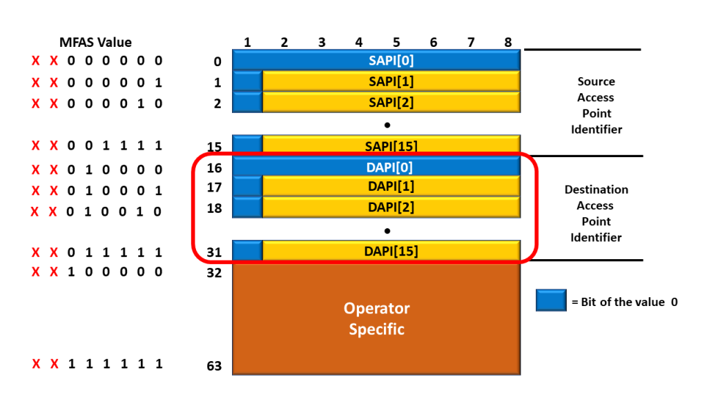
Likewise, for the DAPI (Destination Access Point Identifier) field.
We always transmit the first byte of the DAPI field, DAPI[0] coincident whenever the 6 LSBs of MFAS are [0, 1, 0, 0, 0, 0].
I highlight the 16-byte DAPI field within the TTI Message in Figure 3.
Figure 3, The 16-byte DAPI field.
Access Point Identifier (SAPI and DAPI) Features
Each API (or Access Point Identifier) must have the following features (and I’m quoting ITU-T G.709):
Each API must be globally unique in its layer network.
Where it may be expected that the access point may be required for path set-up across an inter-operator boundary, the access point identifier must be available to other network operators.
The access point identifier should not change while the access point remains in existence.
The access point identifier should identify the country and network operator responsible for routing to and from the access point.
The set of all access point identifiers belonging to a single administrative layer network should form a single access point identification scheme.
The scheme of access point identifiers for each administrative layer network can be independent of the scheme in any other administrative layer network.
The standards recommend that the ODUk, OTUk, and OTS each have the access point identification scheme based on a tree-link format to aid routing control search algorithms. The access point identifier should be globally unambiguous.
Additionally, according to Figures 1, 2, and 3, the network must set the first bit (within each byte of the SAPI and the DAPI) to “0”. Hence, we represent the SAPI and DAPI values with 15 7-bit characters.
What Kind of Data Do We Transport via the SAPI and DAPI Fields within the TTI Messages?
I earlier mentioned the following:
Each TTI Message contains a 16-byte SAPI and 16-byte DAPI field
However, the network set the first byte of each SAPI and DAPI field to an all-zeros pattern.
In the remaining 15 bytes (of the SAPI and DAPI fields), the most significant bit-field is set to “0”.
This means that the SAPI and DAPI fields carry 15 7-bit fields.
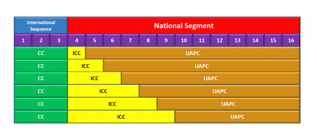
ITU-T G.709 states that “the access point identifier (SAPI, DAPI) shall consist of a three-character international segment (or sequence) and a twelve-character national segment.” I illustrate the basic structure for the Access Point Identifier (SAPI and DAPI) below in Figure 4.
Figure 4, Access Identifier Structure (for both SAPI and DAPI)
The international segment (or international sequence) field consists of a three-character ISO 3166 geographic/political Country Code (G/PCC). The country code (CC) shall be based on the three-character uppercase alphabetic ISO 3166 country code (e.g., USA, FRA).
The national segment field consists of two subfields: the ITU carrier code (ICC) is followed by a unique access point code (UAPC).
The ITU carrier code is a code assigned to a network operator service provider, maintained by the ITU-T Telecommunication Standardization Bureau (TSB) as per ITU-T M.1400. This code shall consist of 1 to 6 left-justified characters, alphabetic, or leading alphabetic with trailing numeric.
The unique access point code shall be a matter for the organization to which the country code and ITU carrier code have been assigned, provided that uniqueness is guaranteed. This code shall consist of 6 to 11 characters, with trailing NUL, completing the 12-character national segment.
Clueless About OTN? We Can Help! Click on the Banner Below to Learn More!
Discounts Available for a Short Time!!
So What Does All This Mean for STE Equipment?
All of this means the following:
Each piece of Section Terminating Equipment (STE) contains a unique 15-character (7-bit) Access Point Identifier value.
In other words, no two STEs (in the world) can share the same 15-character Access Point Identifier value.
The ITU and the nation (that the STE resides within) dictate the exact Access Point Identifier value (that we assign to a given STE).
Whenever a given STE transmits a TTI message to another STE, it will use the SAPI value to identify itself (the Source STE). It will also use the DAPI value to identify the Destination STE (that it sends the TTI Message to).
We Also Deal with TTI Messages with PTE (Path Terminating Equipment) and TCMTE (Tandem Connection Terminating Equipment) – Do These Rules apply to the ODU Layer and the ODUT Layers as Well?
The answer is yes.
Each piece of Path Terminating Equipment (PTE) contains a unique 15-character (7-bit) Access Point Identifier value.
The ITU and the nation (that the PTE resides within) dictate the exact Access Point Identifier value (that we assign to a given PTE).
Whenever a given PTE transmits a TTI message to another, it will use the SAPI value to identify itself (the Source PTE). It will also use the DAPI value to identify the Destination PTE (that it sends the TTI Message to).
Each of the four bullet points (above) applies to as many as 6 ODUT (or Tandem Connection Monitoring) Layers (within the TCMTE).
How About the Operator-Specific Portion of the TTI Message
We have no defined use for the Operator Specific Portion of the TTI Message for the time being. For now, we would reserve this 32-byte field for future use.
Which Byte-Fields Do We Use to Transport the TTI Message within an OTN Signal?
We transport TTI Messages within each of the following OTN Layers:
OTU – Section Monitoring Overhead
ODU – Path Monitoring Overhead, and
As many as 6 Tandem Connection Monitoring Layers (TCM01 to TCM06)
Transporting TTI Messages at the OTU-Layer
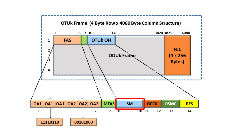
At the OTU Layer, we will use the SM (Section Monitoring) field within each OTU frame to transport TTI Messages. I illustrate an OTU frame with the SM field highlighted in Figure 5.
Figure 5, We Use the Section Monitoring (SM) field to transport the TTI Messages.
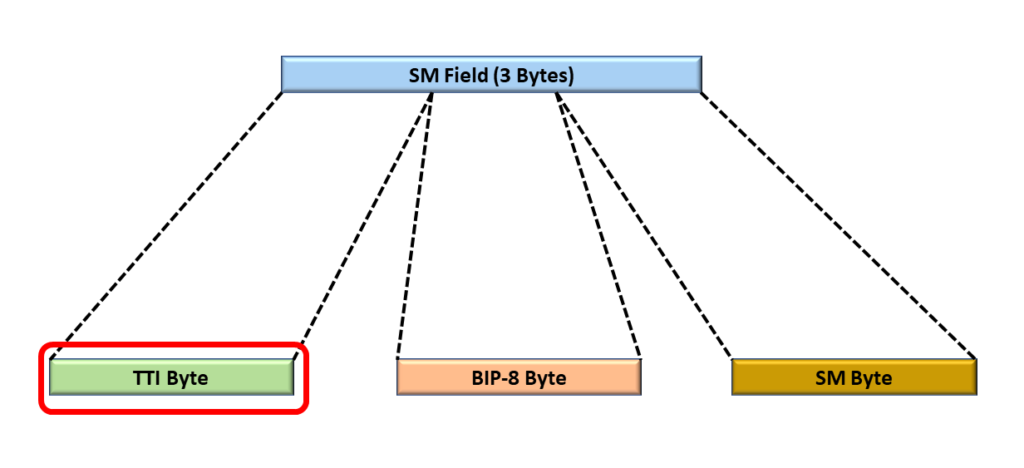
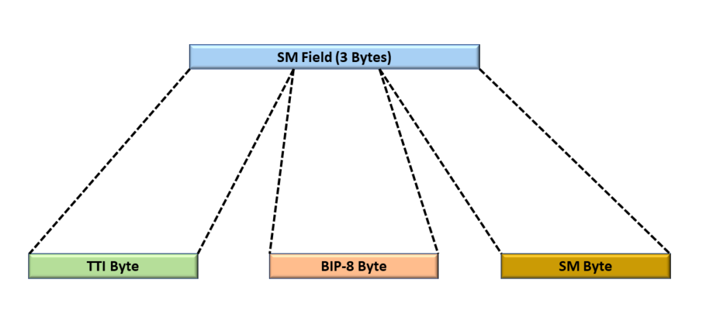
The SM field is a 3-byte field. In Figure 6, I zoom in and expand the SM field (to reveal the 3 bytes within the SM field). We transport the TTI Messages (within an OTU frame) via the TTI byte I show below in Figure 6.
Figure 6, We Identify the TTI (Trail Trace Identifier) Byte within the SM Field – That We Use to Transport TTI Messages via an OTU signal.
Transporting TTI Messages at the ODU Layer
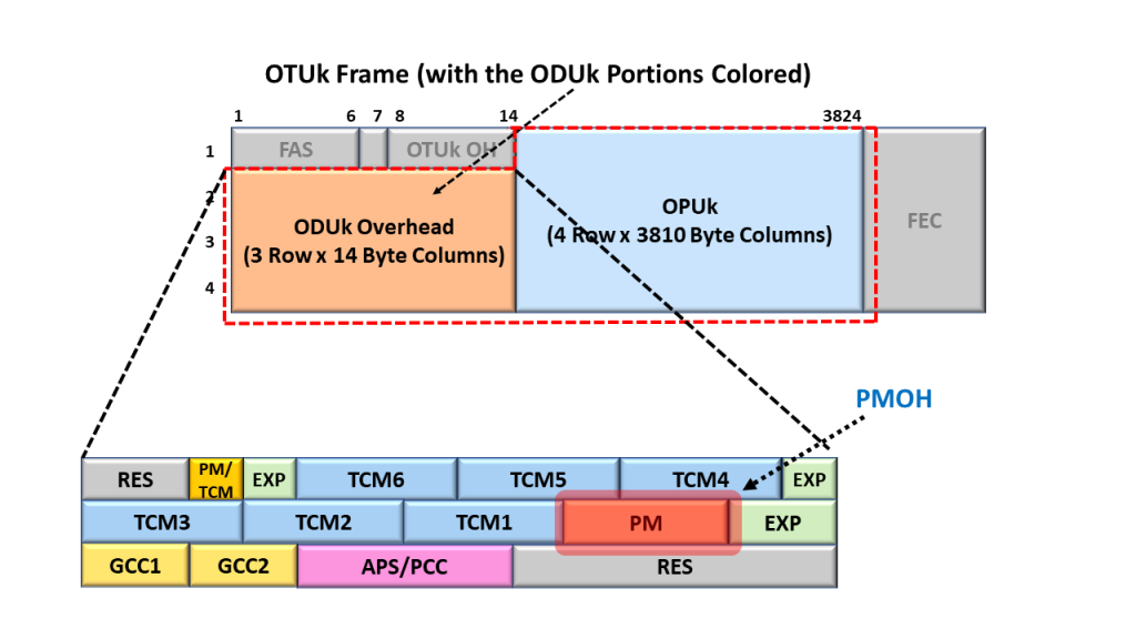
At the ODU Layer, we will use the PM (Path Monitoring) field within each ODU frame to transport TTI Messages. I illustrate an ODU frame with the PM field highlighted in Figure 7.
Figure 7, We Use the Path Monitoring (PM) field to transport the TTI Messages.
The PM field is also a 3-byte field. In Figure 8, I zoom in and expand the PM field (to reveal the 3 bytes within the PM field). We transport the TTI Messages (within an ODU signal) via the TTI byte that I show below in Figure 8.
Figure 8, We Identify the TTI (Trail Trace Identifier) Byte within the PM Field – That We Use to Transport TTI Messages via an ODU signal.
Transporting TTI Messages at (as many as) 6 ODUT Layers – for Tandem Connection Monitoring
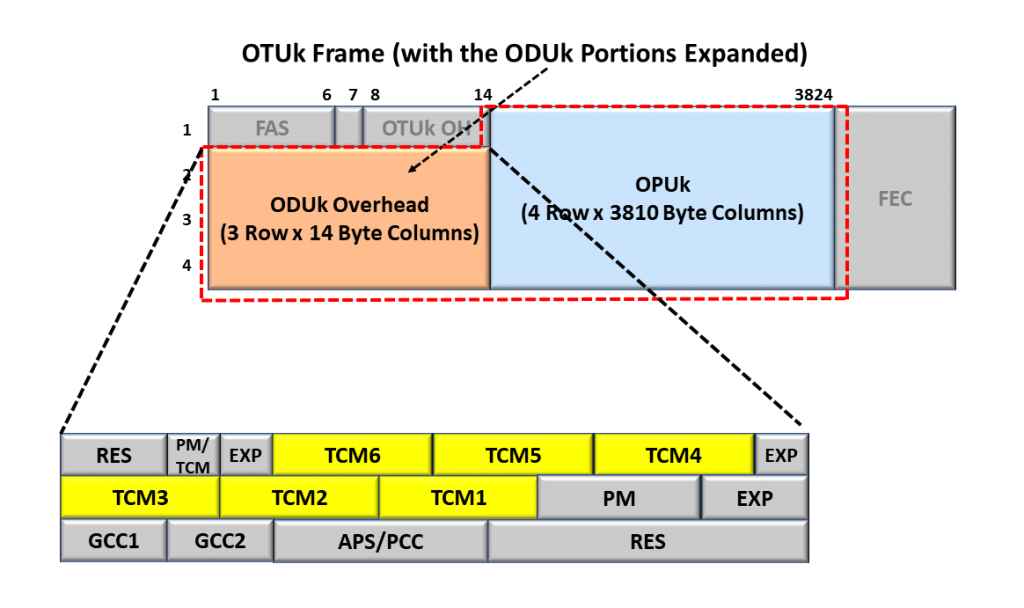
At the ODUT Layers, we will use the SM (Section Monitoring) field within as many as six (6) TCMOH fields within each ODUT frame to transport TTI Messages. I illustrate an ODU/ODUT frame with the 6 TCMOH fields highlighted in Figure 9.
Figure 9, An ODU Frame with each of the 6 TCMOH Fields Highlighted
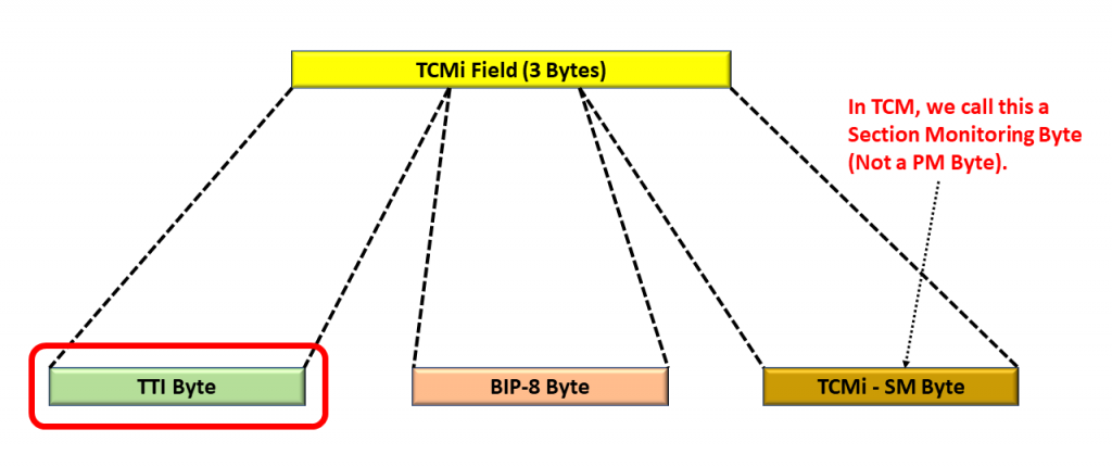
Each of the TCM fields is also a 3-byte field. In Figure 10, I zoom in and expand the TCM field (to reveal the 3 bytes within each TCM field). We transport the TTI Messages (within an ODUT signal) via the TTI byte that I show below in Figure 10.
Figure 10, We Identify the TTI (Trail Trace Identifier) Byte within a given TCM Field – That We Use to Transport TTI Messages via an ODUT signal.
To be clear, we can transport as many as 8 TTI messages independently through an OTN signal at a given time.
One TTI Message at the OTU Layer (via the TTI-byte-field within the SM byte)
One TTI Message at the ODU Layer (via the TTI-byte-field within the PM byte), and
As many as 6 TTI Messages at each (of 6 possible) ODUT/TCM Layers (via the TTI byte-field within the SM byte).
Please see the relevant post for more details on how we transport TTI Messages at a given OTN Network Layer.
This blog post brief defines the term “Section Monitoring Overhead” (SMOH) for OTN Applications.
What Exactly is the OTUk-SMOH (Section Monitoring Overhead)?
Throughout much of this Blog, whenever I discuss Defects or Errors at the OTUk Layer, I usually mention the expression – OTUk-SMOH.
We have also referred to this same field as the Section Monitoring Overhead or SMOH. Each term means the same things; I can use them interchangeably in this blog post.
What exactly is the OTUk-SMOH?
SMOH is an abbreviation for Section Monitoring Overhead.
Figure 1 presents the location of the Section Monitoring (SM) Overhead within the OTU Frame.
Figure 1, Illustration of the OTU Overhead (within an OTU Frame) – with the Section Monitoring Overhead (or SM) Highlighted.
The SM field (or the Section Monitoring Overhead) is a three-byte field. If I were to take that SM field and zoom in on it (to take a closer look), I would have the image below in Figure 2.
Figure 2, Close-Up Look at the SM (or Section Monitoring) field.
Figure 2 shows that the SM field consists of 3-byte fields.
TTI Byte-field
BIP-8 Byte field and
the SM Byte field.
What Are These Byte-Fields Within the SMOH?
Let’s go through and define these byte-fields and the role that they take in Section-Monitoring and Management.
What is the TTI Byte field?
I present an illustration of the SM field with the TTI Byte field Highlighted in Figure 3.
Figure 3, Illustration of the SM Field with the TTI Byte Highlighted
First, “TTI Byte” means Trail Trace Identifier Byte. The purpose of the TTI byte (within the OTUk-SMOH) is to transport the Trail-Trace Identifier Messages from a Source STE to a Sink STE. I show an illustration of the Source STE (STE # 1) transporting the TTI Message to the Sink STE (STE # 2) in Figure 4.
Figure 4, Illustration of a Network Consisting of an STE transmitting the TTI Message to another STE.
Figure 4 illustrates a network that consists of two (2) pieces of equipment:
STE # 1, and
STE # 2
I will briefly define and elaborate on these pieces of equipment.
STE # 1
This piece of equipment accepts an OTU4 signal (as an input) from the left-hand side (of the figure) and ultimately outputs an OTU4 single (at the other end of this equipment) out to STE # 2
STE # 2
This piece of equipment accepts an OTU4 signal (as an input) from STE # 1 and ultimately outputs an OTU4 signal (at the other end of this equipment) out to some off-page STE.
What is the TTI Message?
Without going into the details of the TTI Message (and what it means), we will, for now, say that this is a 64-byte message (16-byte SAPI, 16-byte DAPI, and 32 bytes Operator Specific) that uniquely identifies a particular STE (Section Terminating Equipment). Figure 5 presents the byte format of the TTI Message.
Figure 5, Illustration of the Byte Format of the TTI Message
In this figure, we show that the TTI Message is a 64-byte message that:
Consists of 16 bytes for the SAPI (Source Access Point Identifier)
16 bytes for the DAPI (Destination Access Point Identifier), and
32 bytes for the Operator Specific field.
I will define the SAPI and the DAPI in another post. Another point I will make in Figure 5 is that the transmission of TTI Messages is always synchronized with the MFAS byte-field.
For this blog post, I will say that a given STE (STE # 1 in this case) will use the 64-byte TTI Message to repeatedly identify itself to the other STE (STE # 2). STE # 1 will continually transmit these TTI messages to STE # 2. STE # 2 will ensure that it consistently receives an expected (and correct) TTI Message. In other words, STE # 2 will use these TTI Messages to check and verify that it is connected to the correct STE (STE # 1).
How Do We Use the TTI Bytes to Transport the TTI Messages?
Figure 5 shows that there are 64 bytes within each TTI Message. However, Figure 3 shows only one TTI byte within the SM field (hence, only one TTI byte within an entire OTU frame). Therefore, transporting a single 64-byte TTI message over an OTU Section requires that we transport 1 TTI byte at a time over a set of 64 OTU frames.
Further, Figure 5 shows that we will synchronize our transmission of these TTI bytes with the MFAS byte.
For example, whenever the 6-LSBs of the MFAS is set to [0, 0, 0, 0, 0, 0], then we will transport the very first TTI byte of the 64-byte TTI Message. Whenever the 6-LSBs of MFAS are set to [0, 0, 0, 0, 0, 1], then we will transport the second TTI byte of the 64-byte TTI message, and so on.
The Receiving STE (STE # 2) in Figure 4 will use this relationship between the LSBs of the MFAS byte to interpret the data it receives from the Transmitting STE (STE# 1) in this case.
If the Receiving STE receives an erred (or unexpected) value for the TTI Message, then that STE can declare the dTIM (Trail-Trace Identifier Mismatch) defect. We will discuss exactly how an STE declares and clears the dTIM defect in another post.
Clueless About OTN? We Can Help! Click on the Banner Below to Learn More!
Discounts Available for a Short Time
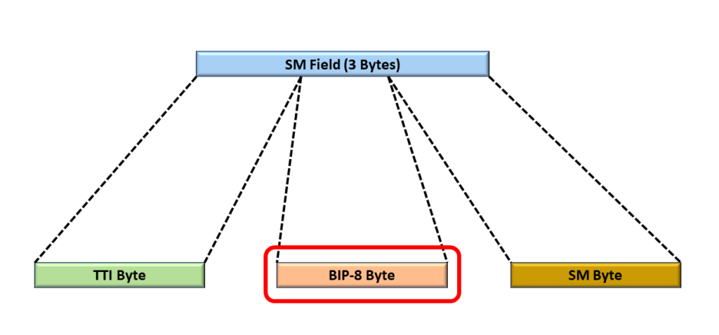
What is the SM-BIP-8 Byte-Field?
I present an illustration of the SM field with the BIP-8 Byte-field Highlighted in Figure 6.
Figure 6, Illustration of the SM Field with the SM-BIP-8 Byte field highlighted.
The purpose of the BIP-8 Byte field is to permit the receiving STE to perform error checking (and reporting) on each OTU frame it receives.
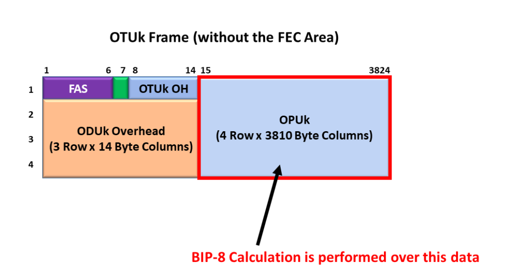
Figure 7, OPU Payload Data that the Transmitting STE uses to Compute the SM-BIP-8 Value
The transmitting STE will then insert this BIP-8 Byte within the BIP-8 Byte (of a specific OTU frame).
Figure 8, Transmitting STE inserting the SM-BIP-8 Value into a Specific Location within the OTU data stream.
The transmitting STE will then transmit this SM-BIP-8 value (along with the rest of the data within the SM field and the OTU data stream) to the remote receiving STE.
As this Receiving STE receives and accepts an OTU data stream, it also locally computes its own value for the SM-BIP-8 byte-field (based on the data within the OPU Payload). The Receiving STE will also read in the SM-BIP-8 value (the transmitting STE computed and inserted into the SM-byte within the OTU data stream).
If the Receiving STE determines that the SM-BIP-8 value (that it reads from the SM field within the OTU data-stream) matches that of its locally computed SM-BIP-8, then it will determine that the Receive STE received an OTU frame in an un-erred manner.
On the other hand, if the Receiving STE determines that the SM-BIP-8 value (that it reads from the SM-field within the OTU data-stream) differs from that within its locally computed SM-BIP-8 value, then it will determine that the Receive STE received some OTU data in an erred manner.
The SM-BIP-8 blog post presents a detailed discussion on how the Transmitting STE computes the SM-BIP-8 value and inserts it into the SM field within the OTU frame.
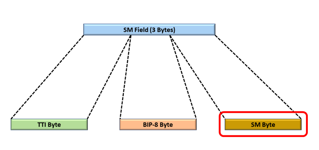
What is the SM Byte field (within the SM field)?
I present an illustration of the SM field with the SM Byte field Highlighted in Figure 7.
Figure 7, Illustration of the SM-field with the SM-byte highlighted
However, if we were to take a closer look at the SM byte (within the SM-byte), we could see that the SM-byte would consist of multiple bit fields, as shown below in Figure 8.
Figure 8, A Closer Look at the SM-byte-field within the SM-field
Figure 8 shows that the SM-byte consists of the following bit or nibble fields.
BEI/BIAE Nibble-Field
BDI bit-field
IAE bit-field
RES field (2 bits in width)
I will briefly define these nibble and bit-fields within the SM-byte field.
The Backward Error Indicator is a four-bit field that reflects the number of SM-BIP-8 errors detected by a Receiving STE (and flagged) within the remote recently received OTU frame. If this nibble field contains a value of 0x00 to 0x08, it is transporting the BEI value for a given OTU frame. Please see the blog post on the SM-BEI nibble field to learn more about this topic.
On the other hand, if the BEI/BIAE contains the value of 0x0B, then this reflects a BIAE (Back Input Alignment Error) condition. Please see the blog post on IAE and BIAE defects to learn more about this topic.
BDI – Backward Defect Indicator bit-field
If the local receiving STE declares a service-affecting defect, it will set the BDI bit-field (that it sends out to the remote terminal) to “1”. On the other hand, if the local receiving STE does not declare a service-affecting defect, it will set the BDI bit-field (that it sends out to the remote terminal) to “0”.
It Receiving STE detects a frame slip event (upstream) within the incoming OTU data stream, then will set this IAE bit-field to “1”.
Please see the blog post on IAE and BIAE defects to learn more about this topic.
Conclusion
I have briefly discussed the Section Monitoring Overhead within this blog post. This write-up was intended to be introductory and kept at a high (and simple) level. Please check out those individual blog posts for more details on how we compute specific SMOH fields. I did not want to repeat this detailed material (calculating the SM-BIP-8 value, the SM-BEI value, etc.) in this blog post.
This blog post presents a video that discusses the APS features within some fo the Atomic Functions that we discussed in Lesson 11.
Lesson 12 – Video 13 – Detailed Implementation of APS within the Atomic Functions – Video 2
This blog post continues our discussion of the APS features within various Atomic Functions. In this case, we will present how to implement Automatic Protection Switching in great detail. In particular, we will describe the following:
APS Features within the ODUT/ODU_A_So and ODUT/ODU_A_Sk functions (ODUT/TCM Layer – SNC/S Monitoring)
How do we implement the APS features within these Atomic Functions to support TCM Layer i SNC/S Monitoring and Protection-Switching?
How do we implement a complete System-Level design (using these atomic functions along with the ODUT_TT_So and ODUT_TT_Sk Atomic Functions)?
NOTE: We discussed these atomic functions in Lesson 11. However, we did not discuss the APS features (within those functions) then.
More specifically, we discuss how our system should implement APS and the APS Communication Protocol whenever the upstream ODUT_TT_Sk Atomic Function declares either a Service-Affecting or the TCMi-dDEG defect.
This blog post presents a video that discusses the APS features within some of the Atomic Functions that we discussed in Lessons 9 and 10.
Lesson 12 – Video 12 – Detailed Implementation of APS within the Atomic Functions – Video 1
This blog post starts our discussion of the APS Features within various Atomic Functions. In this case, we will present how to implement Automatic Protection Switching in great detail. In particular, we will describe the following:
APS Features within the OTUk/ODUk_A_So and OTUk/ODUk_A_Sk functions (OTU-Layer/SNC/I Monitoring)
How do we implement the APS features within these Atomic Functions to support OTU-Layered SNC/I Monitoring and Protection-Switching?
How do we implement a complete System-Level design (using these atomic functions along with the OTUk_TT_So and OTUk_TT_Sk Atomic Functions)?
NOTE: We discussed these atomic functions in Lesson 9. However, we did not discuss the APS features (within those functions) then.
APS Features within the ODUkP/ODUj-21_A_So and ODUkP/ODUj-21_A_Sk functions (ODU-Layer/SNC/I Monitoring)
How do we implement the APS features within these Atomic Functions to support ODU-Layered SNC/I Monitoring and Protection-Switching?
How do we implement a complete System-Level design (using these atomic functions along with the ODUk_TT_So and ODUk_TT_Sk Atomic Functions)?
NOTE: We discussed these atomic functions in Lesson 10. However, we did not discuss the APS features (within those functions) then.
APS Features of the ODUkP/ODUj-21_A_So and ODUkP/ODUj-21_A_Sk functions (CL-SNCG/I Monitoring)
How do we implement the APS features within these Atomic Functions to support CL-SNCG/I Monitoring and Protection-Switching?
How do we implement a complete System-Level design (using these atomic functions along with the ODUk_TT_So and ODUk_TT_Sk Atomic Functions)?
NOTE: We discussed these atomic functions in Lesson 10. However, we did not discuss the APS features (within those functions) then.
This blog post presents a video that concludes our discussion of APS Commands via the APS/PCC Communications Protocol
Lesson 12 – Video 11 – Detailed Discussion of APS Commands – Video 4
This blog post completes our discussion of APS Commands and the APS/PCC Communications Protocol. This video serves as Video 4 in this discussion. This blog post briefly discusses the SD, Manual Switch, Wait-to-Restore (WTR), Reverse-Request (RR), and Do-Not-Revert (DNR) APS Commands.
Additionally, this video defines and discusses the 1 Phase APS Communication, 2 Phase APS Communication and 3 Phase APS Communication Procedures.
Finally, this video will define APS Recovery Time. This video will also present the ITU-T G.873.1 APS Recovery Time Requirements.
More specifically, this video will cover the following topics:
Detailed Topics Discussed
APS Commands (Continued)
SD_W (Signal Degrade in the Working Transport Entity)
SD_P (Signal Degrade in the Protection Transport Entity)
This blog post contains a video that continues the discussion of the APS Commands. This video serves as Video 3 of this series of APS Command videos.
Lesson 12 – Video 10 – Detailed Discussion of APS Commands – Video 3
This blog post continues our discussion of APS Commands and the APS/PCC Communication Protocol. This video serves as Video 3 in this discussion. This blog post discusses completing the Force Switch Commands and the SF (Signal Fail) Commands using the APS/PCC Communication Protocol.
In particular, this video will discuss the following topics:
Executing the Force Switch – Normal Traffic Signal n to Protection (for the 1:N Protection Architecture) – Continued from Video 9
Implementing the Force Switch – NULL Test Signal to Protection Command – another way to resume Normal Operation.
Signal Fail APS Commands
Executing the Signal Fail – Working Transport Entity (SF_W) Command (for the 1+1 Protection Architecture)
How does a given Network Element invoke the SF_W Command?
The Protection Group’s operation during SF_W Command execution.
How do we recover from this Command (for a Reverting System)?
Use of the WTR (Wait-to-Restore) Command
Executing the Signal Fail – Protection Transport Entity (SF_P) Command (for the 1+1 Protection Architecture)
How does a given Network Element invoke the SF_P Command?
The Protection Group’s operation during SF_P Command execution.
How do we recover from this Command?
Executing the Signal Fail – Working Transport Entity (SF_W) Command (for the 1:N Protection Architecture)
How does a given Network Element invoke the SF_W Command?
The Protection Group’s operation during SF_W Command execution.
How do we recover from this Command (for a Reverting System)?
Use of the WTR (Wait-to-Restore) Command.
Executing the Signal Fail – Protection Transport Entity (SF_P) Command (for the 1:N Protection Architecture)
How does a given Network Element invoke the SF_P Command?
The Protection Group’s operation during the SF_P Command execution.
This blog post presents a video that continues our discussion of APS Commands via the APS/PCC Communication Protocol. This video serves as Part 2 of this discussion.
Lesson 12 – Video 9 – Detailed Discussion of APS Commands – Video 2
This blog post continues our discussion of APS Commands and the APS/PCC Communication Protocol. This video serves as Video 2 in this discussion. This blog discussed implementing the LoP (Lock Out of Protection) and Force Switch Commands using the APS/PCC Communication Protocol.
In particular, this video will discuss the following topics:
Executing the LoP (Lock Out of Protection Command) – for both the 1+1 and 1:N Protection Architectures
What does the LoP Command do to the Protection Group?
How do we Implement this Command?
How do we Terminate this Command (to resume Normal Operation)
Executing the Force Switch – Normal Traffic Signal to Protection (for the 1+1 Protection Architecture)
How does this command’s execution affect the Protection Group’s operation?
How do we Implement this Command?
Implementing the Force Switch – NULL Test Signal to Protection Command – to resume Normal Operation.
Executing the Force Switch – Normal Traffic Signal n to Protection (for the 1:N Protection Architecture)
How does this command’s execution affect the Protection Group’s operation?
How do we Implement this Command?
Implementing the Force Switch – Extra Traffic Signal to Protection Command – to resume Normal Operation.
To Learn More About the LoP (Lock Out of Protection) and Force Switch Commands, Check Out the Video Below.
This blog post presents a video that shows how to implement APS (Automati Protection Switching) both with and without using an APS Communication Protocol.
Lesson 12 – Video 8 – Detailed Discussion of APS without and with the APS Communication Protocol – Video 1
This blog post describes how we can implement APS (Automatic Protection Switching) without using an APS Communication Protocol. Afterward, this blog introduces how to implement APS using the APS Communication Protocol. This video serves as the first of several videos on this topic.
In particular, this video will discuss the following topics:
Executing APS without using the APS Communication Protocol
Under what conditions can we implement APS without using an APS Communication Protocol?
Why can we implement APS (without an APS protocol) in this case?
When not supporting an APS Communication Protocol, the Architecture/Design of the Protection-Switching Controllers.
How to implement Automatic Protection Switching – without implementing an APS Communication Protocol.
Executing APS with an APS Communication Protocol
Under what conditions must we implement APS with an APS Communication Protocol?
Why do we need to use an APS Communication Protocol for these cases?
How to implement Automatic Protection Switching – while using an APS Communication Protocol
Introduction to the APS/PCC Field for OTN/Linear Protection Switching Applications (per ITU-T G.873.1).
The Architecture/Design of the Protection-Switching Controllers – 1+1 Protection Architecture
The Architecture/Design of the Protection Switching Controllers – 1:N Protection Architecture
The NR (No Request) Command
To Learn How to Implement APS, with and without an APS Communication Protocol, Check Out the Video Below.
This blog post briefly defines and describes the Nibble and Byte fields of the APS/PCC field, for Linear-Protection-Switching and OTN Applications.
Introduction to the APS/PCC Field
This blog post aims to define and describe the byte format of the APS/PCC field within the ODU Overhead whenever we support Linear Protection Switching applications within the OTN. ITU-T G.873.1 specifies the byte/nibble format of the APS/PCC field that we use within the OTN for Linear Protection Switching.
Whenever the System Designer needs to support the following:
Linear Protection Switching within the Optical Transport Network (defined within ITU-T G.709)
An APS Communication Protocol (because the user is either using the 1:N Protection Architecture or Bidirectional Switching
Then the user will need to use the APS/PCC (Automatic Protection Switching/Protection Control Communications) channel (and field) to support the APS protocol.
The APS/PCC field resides within the ODU Overhead, as I show below in Figure 1.
Figure 1, Location of the APS/PCC Field within the ODU Overhead of an OTU Frame.
Figure 1 shows that the APS/PCC field resides within the fourth row and the fifth through eighth-byte position within an OTU frame. The length of the APS/PCC field is four bytes wide.
Whenever we are designing OTN networks to also support protection switching (and using the APS Communications Protocol) in the process, then we will use the APS/PCC field to transport APS Messages from one Network Element to another.
Byte/Nibble Format of the APS/PCC Field
I show the Byte/Nibble format of the APS/PCC field below in Figure 2.
Figure 2, Byte/Nibble format of the APS/PCC Field
Figure 2 shows that the APS/PCC field consists of the following Nibbles and Byte-fields:
Request/State Nibble (Bits 1-4)
The purpose of this Nibble-field is to either:
Transmit Protection-Switching commands or requests to the remote terminal of the Protection-Group, or
Transmit information about Defect Conditions or States.
Table 1 presents a list of values (within the Request/State Nibble field) and their corresponding Meaning.
Table 1, Standard Values within the Request/State Nibble field and their Corresponding Meaning.
So, for example, if a given Protection Switching terminal needs to transmit the SF Command, it would set the Request/State Nibble (within its outbound APS Message) to [1, 1, 0, 0], as I show in Table 1.
Protection Type Nibble (Bits 5 – 8)
The Protection Type Nibble field occupies the second set of four bits of the APS/PCC field.
The purpose of this nibble-field is to communicate (to the remote end of the Protection Group) many of the governing parameters of our Protection-Switching scheme.
The following table presents a list of the bit-fields within the Protection-Type Nibble and their meaning/description.
Table 2, A List of the Bit-Fields, within the Protection-Type Nibble and their Meaning/Description
Bit A – APS Channel
This bit-field indicates if the Protection Group is either supporting an APS Communication Protocol or not, as I describe below.
0 = No APS Channel (Not using the APS Communication Protocol)
1 = APS Channel (We are using the APS Communication Protocol)
Bit B – Bridge (Permanent)
This bit-field indicates if the Protection Group supports the 1+1 or 1:N Protection Architecture, as I show below.
This bit-field indicates if the Protection Group supports the Revertive or Non-Revertive Operation, as I show below.
0 = Non-Revertive Operation
1 = Revertive Operation
Requested Signal Byte – APS/PCC Field – Byte 2
The Requested Signal byte-field identifies the signal that the Near-End (e.g., the Requesting Terminal) requests to be carried over to the Protection Transport Entity.
Ultimately, we a request at the Far-End Terminal to place the Requested Signal on the Protection Transport Entity, following this Protection Command.
For the 1+1 Protection Architecture
For the 1+1 Protection Architecture, the Protection-Switching Terminal should set this byte-field to “0x01” (for most APS Commands) to denote Normal Traffic Signal # 1. Normal Traffic Signal # 1 is typically the ONLY Normal Traffic Signal in a given direction for a 1+1 Protection Switching Architecture.
For the 1:N Protection Architecture
If the Requesting Terminal wishes to command the remote end to bridge the NULL Test Signal to the Protection Transport entity, it should set this byte-field to 0x00 when issuing an APS command.
Likewise, suppose the Requesting Terminal wishes to command the remote end to bridge the Extra Traffic Signal to the Protection Transport entity. In that case, it should set this byte-field to 0xFF when issuing an APS command.
Finally, suppose the Requesting Terminal wishes to command the remote end to bridge a Normal Traffic Signal to the Protection Transport entity. During a Protection Switching event, it should set this byte-field to the appropriate number (corresponding with the defective Normal Traffic Signal). Valid Numbers for the Requested Byte value range from 0x01 to 0xFE, depending upon which Normal Traffic signal requires Protection-Switching.
Table 2 lists the appropriate Requested Signal Values for the 1:N Protection Architecture.
Table 2, List of Appropriate Requested Signal Values for the 1:N Protection Architecture
Bridged Signal Byte – APS/PCC Field – Byte 3
For this field, the REQUESTING terminal will set this byte-field to the value that identifies which signal this terminal is currently bridging to the Protection Transport entity.
For the 1+1 Protection Architecture
When using the 1+1 Protection Architecture, the Protection-Switching Terminal should set this byte-field to “0x01” (for most APS Commands) to denote Normal Traffic Signal # 1. Normal Traffic Signal # 1 is typically the ONLY Normal Traffic Signal in a given direction for a 1+1 Protection Switching Architecture.
For the 1:N Protection Architecture
If the Requesting Terminal is bridging the NULL Test Signal to the Protection Transport entity, it must set this byte-field to 0x00 when issuing an APS command. The Requesting Terminal tells the remote terminal that it is bridging the NULL Test Signal to the Protection Transport entity.
Likewise, if the Requesting Terminal is bridging the Extra Traffic Signal to the Protection Transport entity, it must set this byte-field to 0xFF when issuing an APS command.
Finally, suppose the Requesting Terminal is currently implementing Protection Switching and is bridging one of the Normal Traffic Signals to the Protection Transport entity. In that case, it must identify that Normal Traffic Signal by setting this byte-field to the appropriate number (corresponding with the defective Normal Traffic Signal). Valid Numbers for the Requested Byte value range from 0x01 to 0xFE, depending upon which Normal Traffic signal requires Protection-Switching.
Table 3 presents a list of the appropriate Bridged Signal Values for the 1:N Protection Architecture.
Table 3, List of Appropriate Bridged Signal Values for the 1:N Protection Architecture
Reserved Byte – Byte 4
This byte-field is reserved for future use/standardization.
Clueless About OTN? We Can Help!! Click Below to Learn More!!
Example of Using the APS/PCC Field for the 1+1 Protection Architecture
Let’s suppose we use the 1+1 Protection Architecture within our Protection Scheme. Further, let’s assume that one of the Network Elements declares the SF_W (Signal Fail within the Working Transport Entity) condition, as shown below in Figure 3.
Figure 3, Tail-End Circuit at NE Z declares the SF_W Condition.
NE Z Sends the SF_W APS Message to NE A
In this case, NE Z (the Network Element declaring the SF_W Condition) will need to send the SF_W APS Command to the remote terminal. I show this APS Command below in Figure 4.
Figure 4, NE Z sending the SF_W APS Command to NE Z.
Please note that (within this APS Command) NE Z is setting the Request Command to [1, 1, 0, 0] to denote that it is transmitting the SF Command.
Further, NE Z is also setting the Protection Type Nibble to information NE A, which is operating with the following Protection-Switching characteristics:
A = 1: We are using an APS Communication Protocol
B = 0: We are using a Permanent Bridge (for a 1+1 Protection Architecture)
D = 1: We are supporting Bidirectional Switching, and
R = 1: We are supporting Revertive Switching
Next, NE Z is setting the Requested Byte to “0x01”. This setting denotes two things:
First, we are declaring the SF condition within the Working Transport Entity. If we set the Requested Byte to “0x00”, this would denote that we are declaring the SF condition with the Protection Transport entity.
Second, we are requesting that the remote terminal (NE A, within Figure 4) should bridge the Normal Traffic Signal (Signal # 0x01) to the Protection Transport entity. (NOTE: Because this is the 1+1 Protection Architecture, we are already permanently bridging the Normal Traffic Signal (0x01) to the Protection Transport entity.
Finally, NE Z is setting the Bridged Byte to “0x01”. This setting denotes that we are already bridging the Normal Traffic Signal (0x01) to the Protection Transport Entity. The Permanent Bridge is inherent to the 1+1 Protection Architecture.
Subsequent APS Commands
NE A and NE Z will exchange more APS Commands to deal with this instance of the SF condition. I’m only showing the initial request from NE Z to NE A.
Example of Using the APS/PCC Field for the 1:N Protection Architecture
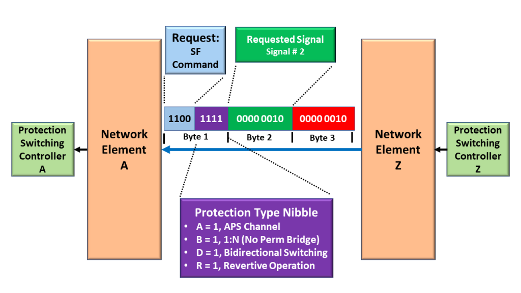
Let’s suppose we are using the 1:N Protection Architecture within our Protection Scheme. Further, let’s assume that one of the Network Elements declares the SF_W Condition with Working Transport Entity # 2, as I show below in Figure 5.
Figure 5, Tail-End Circuit at NE Z declares the SF_W Condition for Working Transport Entity # 2.
NE Z Send the SF (within Normal Traffic Signal # 2) Message to NE A
In this case, NE Z (the Network Element declaring the SF_W Condition) will need to send the SF_W APS Command to the remote terminal. I show this APS Command below in Figure 6.
Figure 6, NE Z sending the SF_W APS Command to NE Z.
Please note (again) that (within this APS Command) NE Z is setting the Request Command to [1, 1, 0, 0] to denote that it is transmitting the SF Command.
Further, NE Z is also setting the Protection Type Nibble to information NE A, which is operating with the following Protection-Switching characteristics:
A = 1: We are using an APS Communication Protocol
B = 1: We are using a Non-Permanent Bridge (for a 1:N Protection Architecture)
D = 1: We are supporting Bidirectional Switching, and
R = 1: We are supporting Revertive Switching
Next, NE Z is setting the Requested Byte to “0x02”. This setting denotes two things:
First, we are declaring the SF condition within the Working Transport Entity. If we set the Requested Byte to “0x00”, this would denote that we are declaring the SF condition with the Protection Transport entity.
Second, we are requesting that the remote terminal (NE A, within Figure 5) should bridge the Normal Traffic Signal # 2 (Signal # 0x02) to the Protection Transport entity. We are declaring the defect with Working Transport Entity # 2. We need to alert the remote terminal that we need to bypass this signal path.
Finally, NE Z is setting the Bridged Byte to “0x02”. This setting denotes that we are already bridging the Normal Traffic Signal # 2 (0x02) to the Protection Transport Entity.
Subsequent APS Commands
NE A and NE Z will exchange more APS Commands to deal with this instance of the SF condition. I’m only showing the initial request from NE Z to NE A.
Has Inflation got You Down? Our Price Discounts Can Help You Fight Inflation and Help You Become an Expert in OTN!! Click on the Banner Below for More Details!!
Click on the Image Below to see more Protection-Switching related content on this Blog: